Age reliability patterns, also known as failure patterns, refer to the trends and behaviors of a system’s reliability and probability of failing as it ages over time. These patterns are crucial in reliability engineering for assessing the performance and lifespan of products, components, or systems. In the 1970s, F. Stanley Nowlan and Howard F. Heap published “Reliability-centered Maintenance” (RCM), a report that significantly changed the industry’s understanding of maintenance, and brought the concept of reliability to the forefront of maintenance programs.
Before RCM, maintenance programs were predominantly based on a belief that most components and assets had an expected lifetime, and that replacing or overhauling these at fixed intervals before the end of that life would prevent unexpected failures. Nowlan and Heap’s published study disproved this belief, and actually found that fixed-interval overhauls in most cases caused more failures than they were preventing. Their research found that a majority of components were most likely to fail right after installation (infant mortality), or at random—with a mere 11% of studied assets benefitting from a limit on operational age.
The study concluded that there were no fewer than six age-reliability/conditional probability of failure relationships that cover the total expected possibilities of failure.
What are the Six Failure Patterns?
*Note the following percentages are based on Nowlan & Heap’s study.
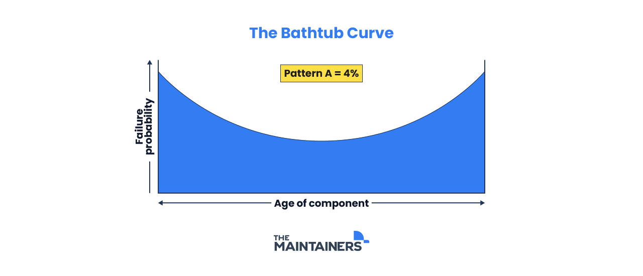
A: The Bathtub Curve
This is the most recognizable failure pattern and depicts three distinct stages: an elevated infant mortality rate, a normal life phase of constant failure probability until the failure probability increases at the end of the item’s lifetime, known as the wear-out phase. This curve encompasses approximately 4% of all failures.
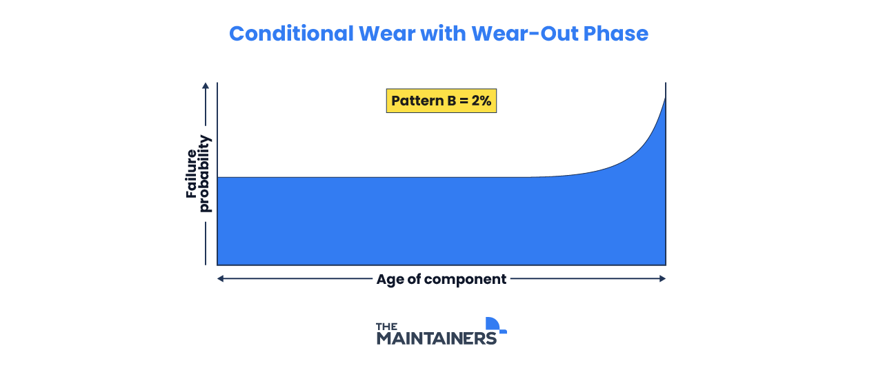
B: Conditional Wear with Wear-Out Phase
This pattern depicts a consistent failure probability until it begins to increase towards the end of its estimated lifetime (wear-out phase); it is similar to the bathtub curve, without the high infant mortality rate. Replacing parts before the expected wear-out phase improved an asset’s reliability. This type of failure is expected for about 2% of all components.
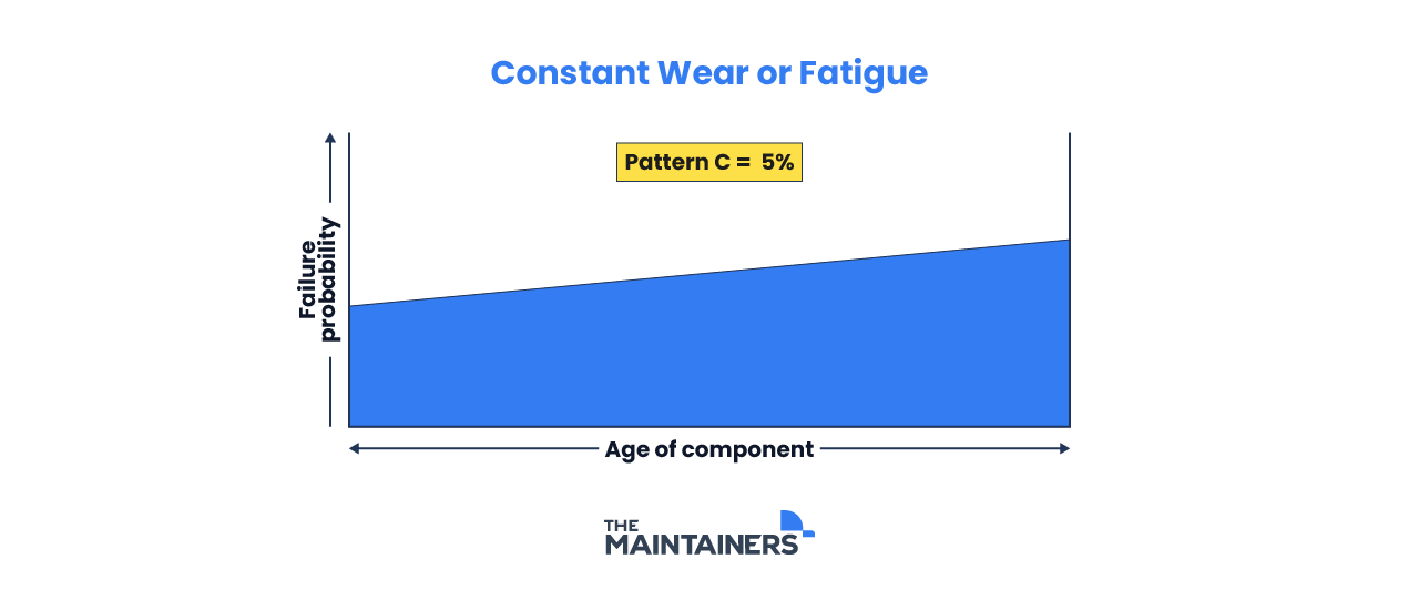
C: Constant Wear or Fatigue
This relationship shows an increasing failure probability with no identifiable wearout age. As there is no clearly defined wear-out point, part replacement happens when the probability has reached a point unacceptable to your operation. This type of failure happens to approximately 5% of components.
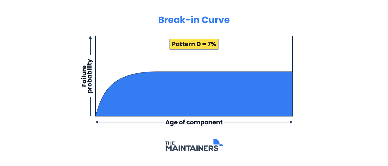
D: Break-in Curve
This failure pattern depicts a low failure probability during initial implementation or installation that eventually increases to a constant level early in its life. As the component has a low probability of failure for only a small percentage of its lifespan, there is no value in replacing this component in a reliability sense. This curve reflects about 7% of all failures.
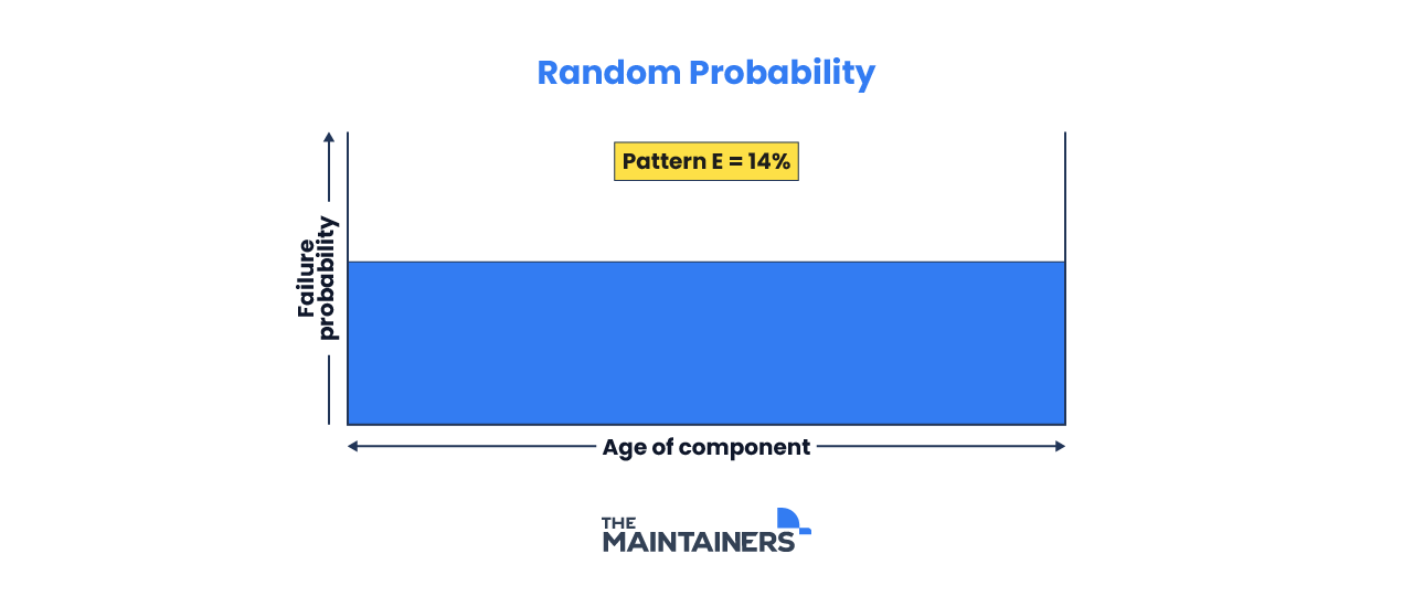
E: Random Probability
This pattern has no changes throughout its lifetime and shows a constant probability of failure. This means failure can randomly happen at any point of its life, and accounts for 14% of all failures.
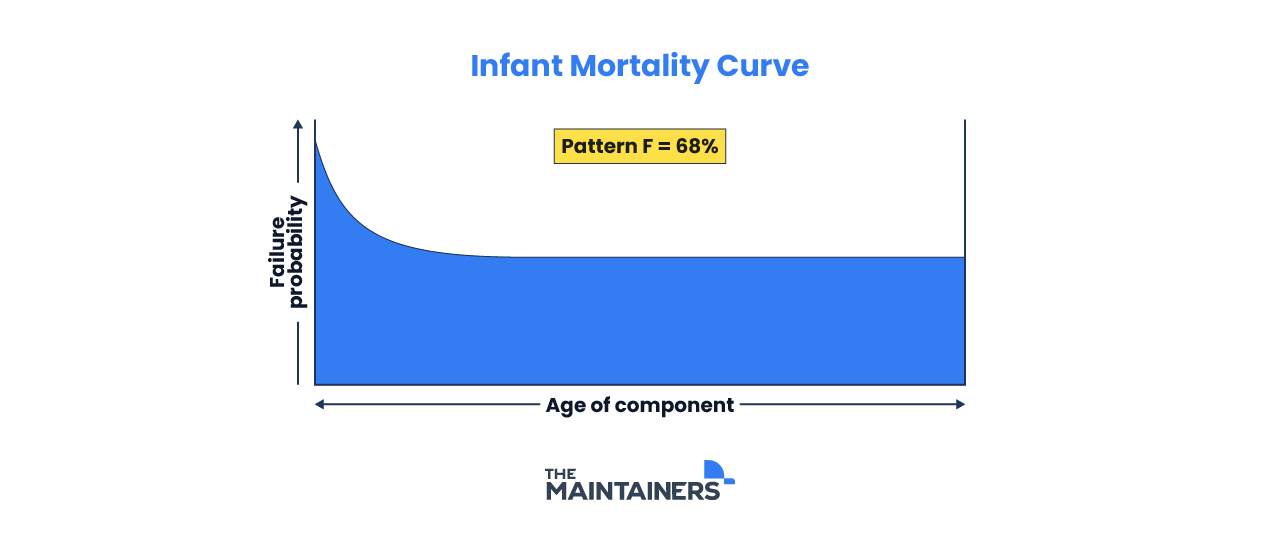
F: Infant Mortality Curve
This is the most likely cause of failure and depicts an elevated probability of failure during a component’s initial installation and use. This probability drops and settles into a constant level for the remainder of its lifespan. This high infant mortality rate is usually due to defects, production mistakes, and human error. This type of failure accounts for 68% of component failures.
Age vs. Random Failures
Of the six above failure patterns, only three (A, B, and C) reflect a direct relationship between an increase in age/time and increased chance of failure. We can categorize these three as “age-related” failure patterns (totalling approximately 15% of all failures), and are the three types of relationships in which machine and asset reliability would benefit from having components replaced after a defined period of time.
Failure patterns (D, E, and F) that reflect random probabilities of failure represent approximately 85% of all failures. To tackle this majority case issue and improve asset reliability despite the “random” odds of failure, we use the P-F model.
What is the P-F Model?
The P-F model is a concept used in the field of condition-based maintenance, which is a strategy for maintaining equipment based on its actual condition rather than a predefined schedule. “P-F” stands for “Potential Failure” and “Functional Failure,” and is defined below.
Potential Failure (P): The stage where there are detectable signs or indicators that suggest a component or system is deteriorating and might fail in the future. However, it hasn’t failed yet, and the equipment is still functioning as expected.
Functional Failure (F): This is the point at which the component or system no longer performs its intended function. In other words, it has failed.
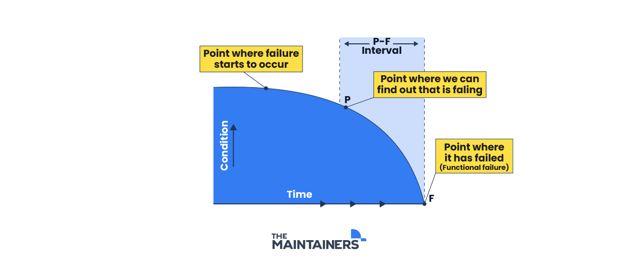
The goal of the P-F model is to detect the potential failure (P) before it progresses to a functional failure (F). This allows maintenance teams to intervene and perform necessary repairs or replacements before a critical failure occurs.
Implementing the P-F model involves using various condition monitoring techniques and technologies to identify the early signs of potential failure. These could include things like vibration analysis, thermography, oil analysis, and other predictive maintenance tools.
Learn more about TRACTIAN’s vibration and temperature monitoring sensor, Smart Trac.
With today’s advancement in technology, condition based monitoring tools can be remotely connected to an enterprise asset management (EAM) system that refines and analyzes the real-time data being collected. By referencing historical data, the system can alert maintenance teams and technicians when an anomaly or error occurs, signaling issues or imminent failure and allowing for preventive maintenance teams to stop the issue in its tracks before any unexpected downtime.
